Principal Component Analysis - A Primer

Principal Component Analysis is a dimension reduction technique. It takes a set of variables, looks for relationships between them, and tries to use those relationships to hopefully help us produce a smaller set of components that we can use in our analysis. In the following I’m going to give some basic detail on how it achieves this, and what these components are, using a simple example.
A Simple Example
Imagine we have a collection of some objects - it doesn’t matter what they are. We have a weighing scale and a measuring tape, and we can measure only two variables about each object - its weight and its length. In the following graph, I’ve plotted the weight versus length for our collection objects.
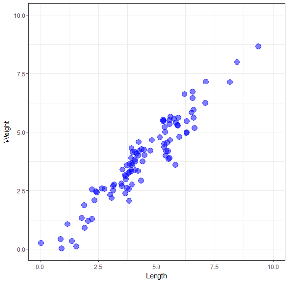
One thing we notice immediately is that they appear to be highly correlated - all the points fall approximately along a straight line. For the sample points, the correlation is 0.95. Since the two variables are so highly correlated, when we know the value of one variable, we can make an excellent guess at the value of the other one. So we don’t really have two different pieces of information about each object. If, for example, we know the weight of an object, we can get a reasonable estimate of its length form the graph (or from building a linear regression model). So actually measuring the length of the object only gives a small bit of extra information - the error in our estimate, which should be small given the two variables are so highly correlated. We could now decide to only use one of these variables in our analysis as including both would not tell us anything extra - we can translate anything we learn from one variable to the other.
This is all relatively straightforward in this simple example, but as we include more variables in our data we have to consider far more relationships between variables and sets of variables. This is where PCA comes in. It helps us achieve the same reduction in a more rigorous way. Let us continue to use our simple data set to see how PCA works.
Extracting the Components
Now that we have our data plotted imagine drawing a new set of axes on top of this data and measuring the distance from each point to the new set of axes, just like in the following graph. We end up with each object measured on these two new variables, which we could use in place of our original two variables. We haven’t lost any, but it would be challenging to interpret our analysis in real-world terms using these two new random axes.
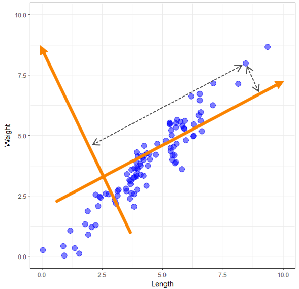
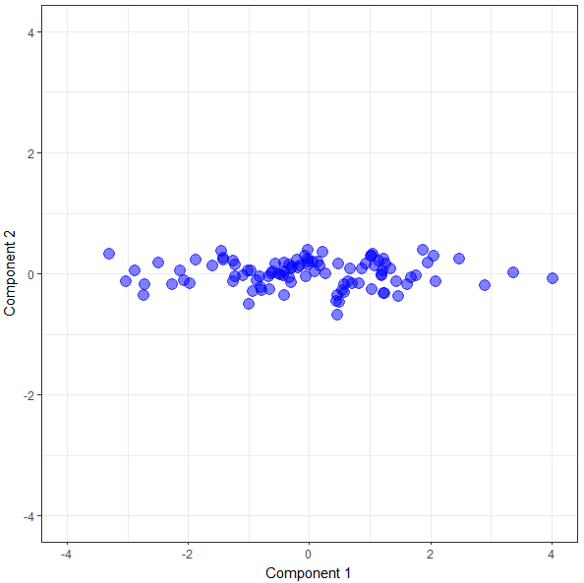
PCA creates a new set of axes, but it doesn’t just draw any random set. It finds the best set subject to some given criteria. There is lots of detail in here that I’m glossing over but understanding this should be sufficient for the rest of what we do. These new axes are the new components we mentioned earlier. We have two variables in our sample data, so we end up with two components. If we had 13 variables, PCA would generate 13 components. So how do these new components help us? In the following graph, I’ve plotted our sample data points on the two components given to us by PCA. Notice how the data is still all spread out along a line but that line is now pretty much horizontal.
Reducing the Dimensions
Let’s look at the variance of the data points on our original metrics and on our new components to see how things have changed. The variances of the length and weights of the objects are 2.89 and 2.92 respectively. We can think of the variance of a variable as how much information that variable contains. For example, if the variance is small, then all the points are close to the mean value, and if you know the mean, you have an excellent approximation for all the data points. If the variance is large, then merely knowing the mean is not a very accurate approximation of all the individual data points.
Taking the variance of our two original variables we can measure what percentage of the total variance each contains. The Length explains 49.7% of the total variance, and the Weight explains 50.3%. (I had already scaled the original variables so this was a simple calculation in this case.) Now if we measure the variance on our new components, we get 1.96 for Component 1 and 0.05 for Component 2. That means that Component 1 contains 97.5% of the variance. In other words, this single component captures 97.5% of the information obtained in the data. Concentrating the variance from across the original variables on to some smaller subset of components is one of the criteria of PCA. We get some components with a lot of the variance and some with very little. The components are ordered from highest to lowest variance so the first or principal component will always have the highest variance.
A step that we can now take is to drop the second component as it doesn’t contain much information. In more technical terms, we tend to keep all components that have an eigenvalue (variance) greater than 1. In our data, only the first component has a variance greater than 1, so we retain it and discard the other. We have now gone from working with two variables to working with only one component, simplifying any analysis we have to do. When we have large sets of correlated variables, this can help us streamline and reduce the dimensions (number of variables/columns) of the data. This is why PCA is known as a dimension reduction technique.
Interpreting the Components
However, how do we interpret our single new component? If we use it in our analysis, then how do we translate what we find in the real world? PCA produces something known as a pattern matrix. This tells us how the original variables are related to the components, and using it, we try to find an interpretation for the component in terms of how it refers to the original variables. We generally put some cutoff on the values in the pattern matrix and ignore any values whose absolute value is less than the cutoff. This approach is beneficial with larger datasets. Typical cutoff values of 0.3 or 0.4 are used. In our simple case, both values are above these thresholds. Our pattern matrix (below) tells us that Component 1, our principal component, is equally dependent (or loaded) on our two variables, length and weight.
| Component 1 | |
|---|---|
| Length | 0.707 |
| Weight | 0.707 |
A label we could give this new component is size. It is an equal mix of the two original variables which are highly correlated to each other. When we measured either one, we essentially measured both as they were so related. The hidden (or latent) aspect of the object that we were measuring was their size. We couldn’t measure the size directly; we could only measure aspects related to it, but PCA help us uncover this.
Hopefully this brief overview illustrates how PCA can help us, not only to reduce the dimensionality of our dataset, but also to find the underlying hidden or latent structure that can exist behind our data.